Benchmark Results
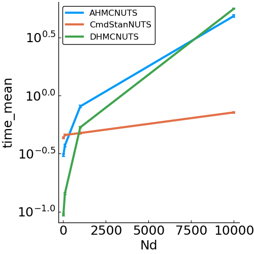
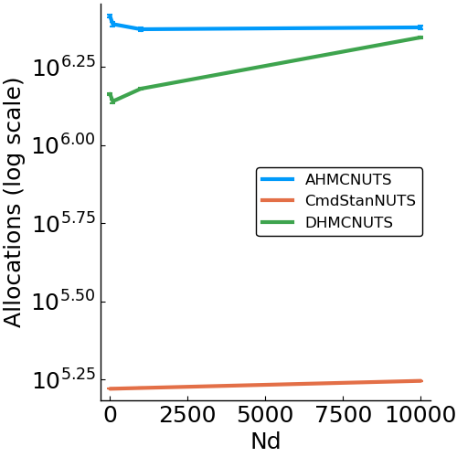
In this section, we report key benchmark results comparing Turing, CmdStan, and DynamicHMC for a variety of models. The code for each of the benchmarks can be found in the Examples folder, while the corresponding code for the models in folder named Models. The benchmarks were performed with the following software and hardware:
- Julia 1.2.0
- CmdStan 5.2.0
- Turing 0.7.0
- AdvancedHMC 0.2.6
- DynamicHMC 2.1.0
- Ubuntu 18.04
- Intel(R) Core(TM) i7-4790K CPU @ 4.00GHz
Before proceeding to the results, a few caveats should be noted. (1) Turing's performance may improve over time as it matures. (2) memory allocations and garbage collection time are not applicable for CmdStan because the heavy lifting is performed in C++ where it is not measured. (3) Compared to Stan, Turing and DynamicHMC exhibit poor scalability in large part due to the use of forward mode autodiff. As soon as the reverse mode autodiff package Zygote matures in Julia, it will become the default autodiff in MCMCBenchmarks.
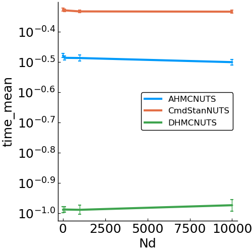
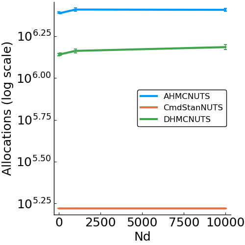
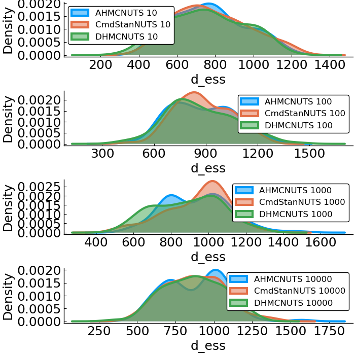
Gaussian
- Model
- benchmark design
#Number of data points
Nd = [10, 100, 1000, 10_000]
#Number of simulations
Nreps = 50
options = (Nsamples=2000, Nadapt=1000, delta=.8, Nd=Nd)- speed
- allocations
- effective sample size
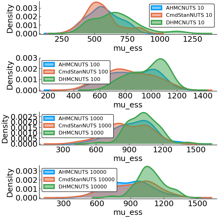
Signal Detection Theory
- Model
- benchmark design
#Number of data points
Nd = [10, 100, 1000, 10_000]
#Number of simulations
Nreps = 100
options = (Nsamples=2000, Nadapt=1000, delta=.8, Nd=Nd)
#perform the benchmark- speed
- allocations
- effective sample size
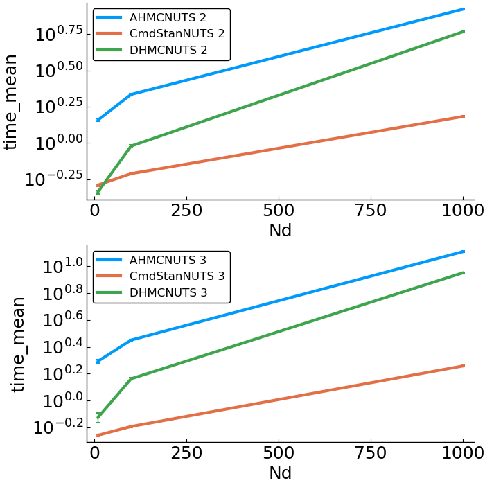
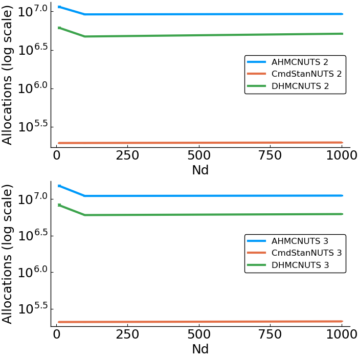
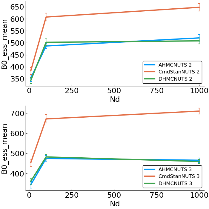
Linear Regression
- Model
- benchmark design
#Number of data points
Nd = [10, 100, 1000]
#Number of coefficients
Nc = [2, 3]
#Number of simulations
Nreps = 50
options = (Nsamples=2000, Nadapt=1000, delta=.8, Nd=Nd, Nc=Nc)- speed
- allocations
- effective sample size
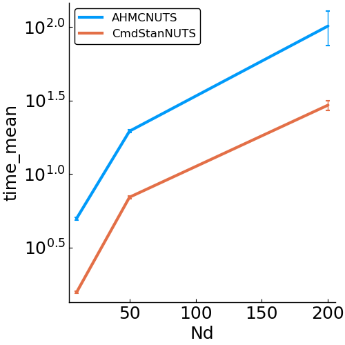
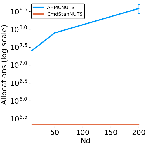
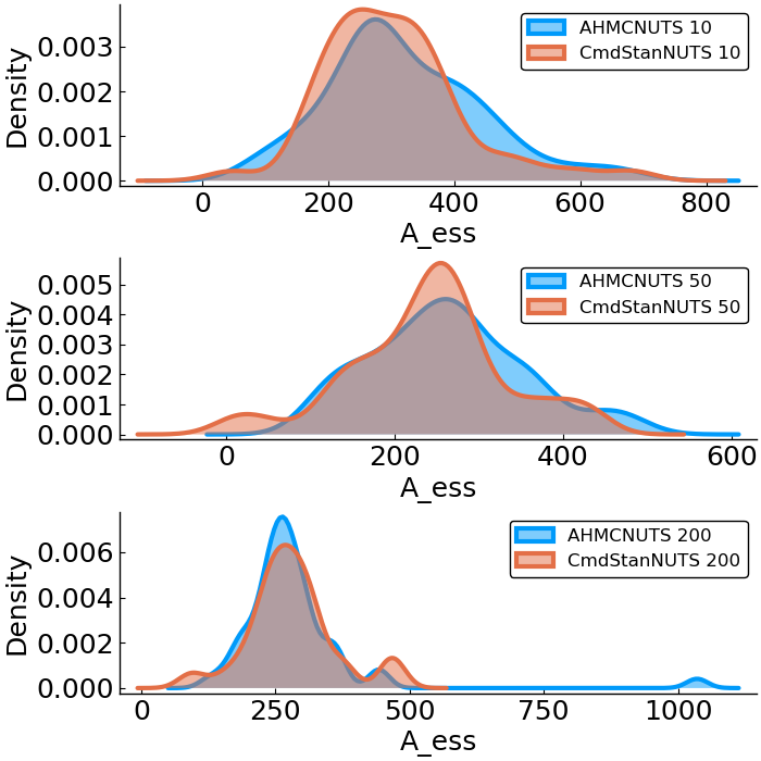
Linear Ballistic Accumulator (LBA)
- Model
where
- benchmark design
#Number of data points
Nd = [10, 50, 200]
#Number of simulations
Nreps = 50
options = (Nsamples=2000, Nadapt=1000, delta=.8, Nd=Nd)- speed
- allocations
- effective sample size
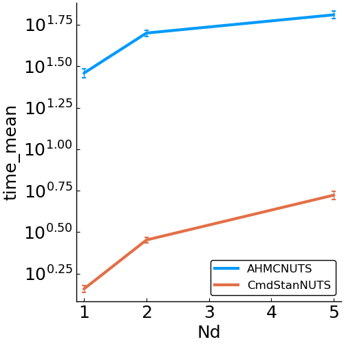
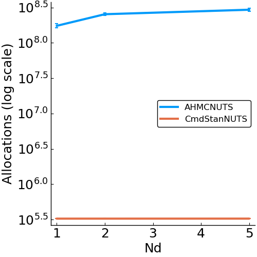
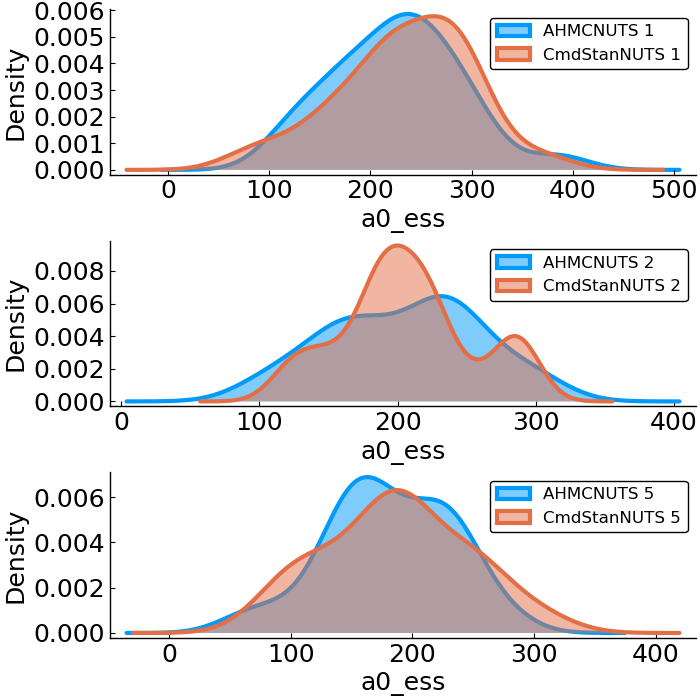
Poisson Regression
- Model
- benchmark design
# Number of data points per unit
Nd = [1, 2, 5]
# Number of units in model
Ns = 10
# Number of simulations
Nreps = 25
options = (Nsamples=2000, Nadapt=1000, delta=.8, Nd=Nd, Ns=Ns)
- speed
- allocations
- effective sample size
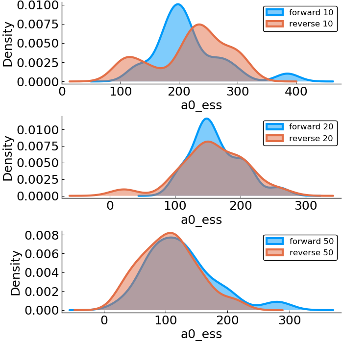
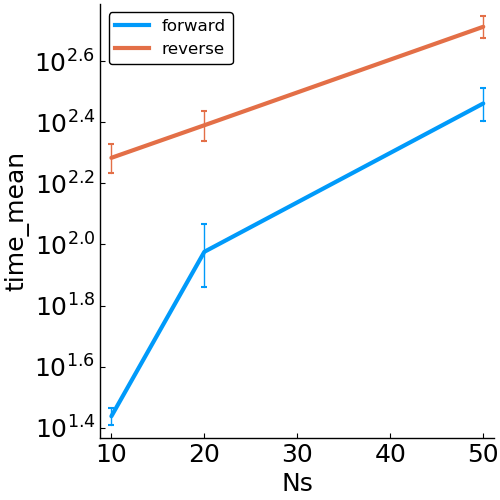
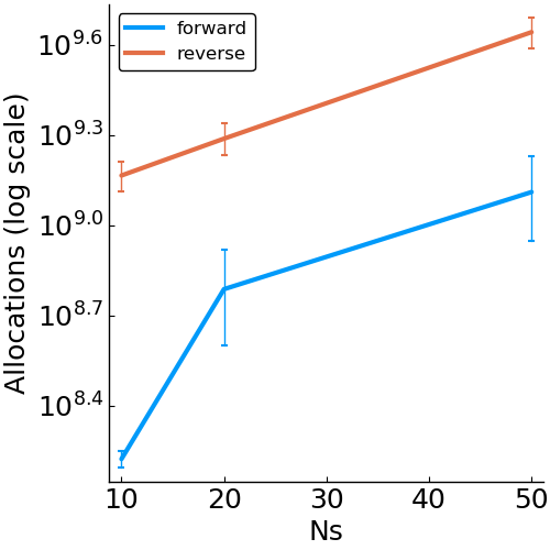
Forward vs. Reverse Autodiff
Hierarchical Poisson
benchmark design
# Number of data points per unit
Nd = 1
# Number of units in model
Ns = [10, 20, 50]
# Number of simulations
Nreps = 20
autodiff = [:forward, :reverse]
options = (Nsamples=2000, Nadapt=1000, delta=.8, Nd=Nd, Ns=Ns, autodiff=autodiff)
- speed
- allocations
- effective sample size